Continuous monitoring
The seismic monitoring of slope conditions is facilitated by a seismic data logger that has been specifically designed to detect ground vibrations, associated with both slope movement and background noise associated with ground layers and properties. A high fidelity 3-component geophone is used to detect ground motion in each of three mutually orthogonal directions and is not affected by lighting conditions or visibility as with the movement detection approach.
Two versions of the data logger and associated telemetry solutions were developed, one that enables continuous monitoring of the slope for landslide detection and the other that is capable of recording higher fidelity data, but is only activated for discrete periods to enable the monitoring of ground conditions (principally ground saturation).
Event Monitoring Data Logger
The continuous monitoring datalogger samples the geophone analogue signals after high frequencies are eliminated using an analogue anti-alias filter at 400 samples every second on each of its three channels and records it to a multi-media card located in the data logging node. A decimated version of the data sampled at 100 samples per second is streamed to the cloud via Google Services. Despite its capabilities, the potential of the datalogger is currently constrained by two significant factors: the need for a substantial power source due to its continuous operation and streaming telemetry, and the limited availability of reliable 4G services on the slope, which can hinder the system’s performance and deployment location. Nevertheless, with appropriate management of these factors, neither of which is an intractable problem, the datalogger can provide valuable seismic data for continuous slope monitoring and related applications.
Event Monitoring Application
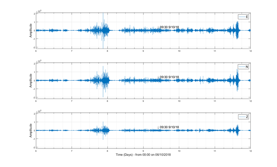
The slope can be monitored to detect landslide events and to track their progression of a landslide event down the slope using the 3-component geophone and continuous monitoring seismic data acquisition node. Figure 11, shows 3-component data recorded from the slope above the Rest and Be Thankful road section over a 12 day period from 00:00 hours on the 6th of October 2018. The two horizontal components are oriented in the east (E) and north (N) directions, orthogonal to the vertical component (Z). The seismicity measured on the slope can be used to detect landslide events and to track their progress down the slope, providing a real-time warning of landslide activity. The geophone seismic system provides continuous slope monitoring capability.
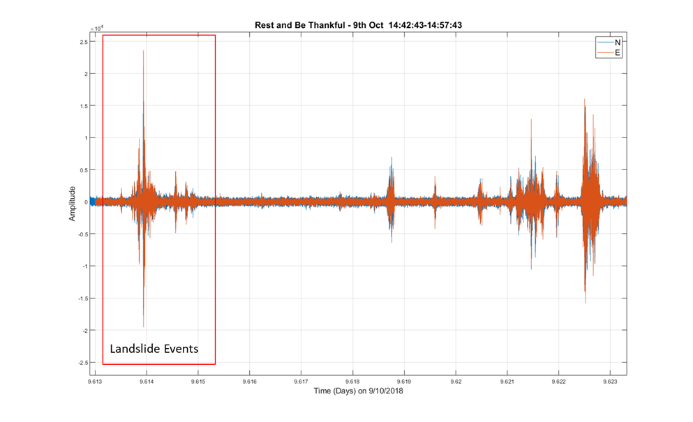
Detection and tracking of landslide events is best achieved by monitoring the two horizontal geophone signals. Figure 12 shows example seismic data from a real and verified landslide activity recorded by the N and E horizontal geophone components on the 9th of October 2018, between 14:42:43 and 14:57:43 hours [the events seen on figure 3 at later times are also landslide events, but the hodogram analysis has only been conducted on the primary initial event in this report]. The amplitude of the seismic events can be used to define a threshold to signify the detection of a landslide event and trigger a warning to the A83 road operators.
The three minute period from 14:42:43 is further analysed in Figure 13 through the use of hodograms.
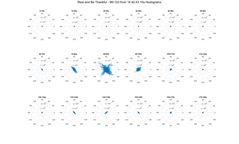
The amplitudes of the E and N geophone signals for a common time sample can be treated as ordinates, to form a 2 dimensional co-ordinate system. If the E ordinate is plotted in the X direction of a graph and the N ordinate is plotted in the Y direction of a chart, the plotting of E and N co-ordinates for successive time samples traces a hodogram figure. Seismic signals are often rectilinear (they form almost straight line shapes within a hodogram) and their resulting hodograms trace linear figures that point in the direction of the source of the signal. The hodograms in Figure 13 are each formed from 10s of data. The major seismic events within the red box from Figure 12 are seen to exhibit rectilinear behaviour and they point in the direction from which the seismic signal originates relative to the sensor. Note that those directions are sometimes different for adjacent hodograms; indicating different parts of the slope are sliding at different times (e.g. row 2, columns 2, 3 and 4). The hodogram sequence in row 2, columns 2, 3 and 4 indicate two landslide events that occurred within the 30s monitoring period. Firstly, we have the landslide with events aligned NW-SE on row 2, columns 2 and 3 and then a later landslide aligned NE-SW in row 2, columns 3 and 4. The amplitude of the rectilinear events on the hodogram from row 2, column 3 are high because the landslide events are closest to the geophone position within that time period. The two events are superimposed on one another in hodogram row 2, column 3, as they are both active within the 10s period monitored by that hodogram. Use of at least two geophones at different locations on the slope can accurately track the progression of a landslide through triangulation of their hodograms from common events.
Ground Condition Monitoring Node Design
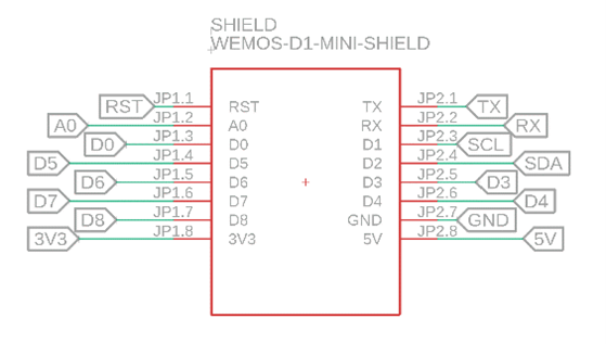
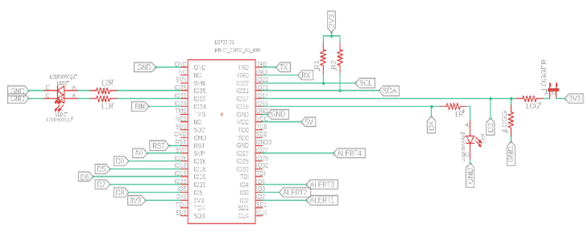
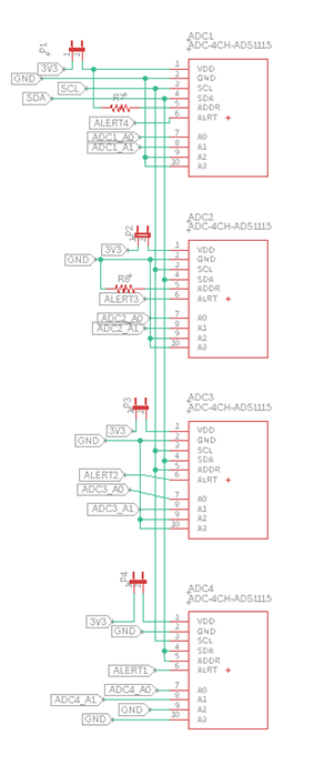
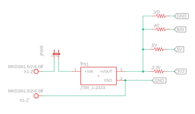
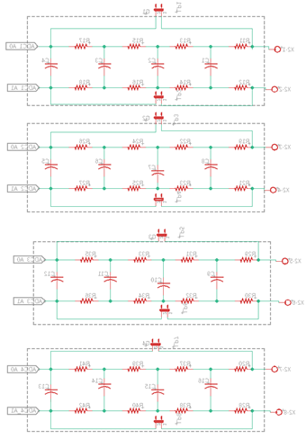
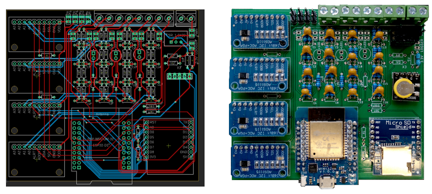
To circumvent the challenges posed by limited 4G connectivity and power requirements, a different version of the datalogger was developed with enhanced capabilities. This new system has an external Real Time Clock for timekeeping control and is designed to sample data at twice the data rate of its predecessor, collecting half an hour of records every 6 hours and uploading the data files to the cloud. This is followed by enabling the sleep mode to conserve power. To further optimize power usage, a relay-based system was designed to only activate the WiFi router when new data are available for upload. This updated datalogger design enables the telemetry of true 800 samples on each channel as were recorded by the node. The schematic, printed circuit board drawing and actual node are given in Figure 14 and Figure 15.
Figure 14. Schematics of Seismic Monitoring Node
Ground Condition Monitoring Application
The discrete period monitoring data logger can be configured to be live for planned discrete periods and to be in sleep mode at other times. Such an operational configuration cannot be used to continuously monitor for landslide events but is ideal for near surface condition monitoring where changes are slower and more progressive. Ground condition monitoring has strong potential as a key indicator of failure potential on the slope and is potentially a key missing dataset in monitoring presently conducted at the site. The primary technique for ground condition monitoring is horizontal-to-vertical spectral ratio analysis (HVSR). The HVSR measures the dynamic characteristics of the subsurface using microtremor measurements propagating through the near-surface ground layers. Microtremors are small, barely noticeable seismic waves constantly passing through the earth's surface, the sources of which are ambient. HVSR analysis calculates the ratio of the amplitude of the horizontal and vertical components of these seismic waves in the frequency domain. The resonance frequencies and amplification factors of these tremors can be calculated to assess the response of the soil strata. The resulting HVSR(f) spectrum is plotted as a function of frequency where the peak frequency fo corresponds to the fundamental resonance frequency of the site and the amplitude of the curve at fo corresponds to the amplification factor. The use of HVSR for slope stability centres on the resonant response of the unconsolidated soil layer being sensitive to its water saturation. The unconsolidated layer thickness above the bedrock on the slope will be constant. The shear-wave velocity in this unconsolidated layer is dependent on the water saturation of the layer, which in turn affects the resonant frequency of the HVSR spectrum. We can monitor the HVSR resonant peak and use the information as a proxy for water saturation. The water saturation of the unconsolidated layer can rise to the point whereby the soil loses its shear strength and the slope will then be prone to sliding.
The use of electroseismic sensors for near surface condition monitoring has been the subject of recent research at Northumbria University. Electroseismic measurements involve deploying an electrode pair into the near surface to be monitored. The electro-potential between electrodes is measured and recorded at a high data sampling rate using the data logger. The incident passive seismic signals measured and analysed using the HVSR approach described above also generate time varying, dynamic electro-potential signals in the near-surface caused by movement of the water within the soil matrix. These dynamic electro-potential signals are detected by the electroseismic sensors. The amplitude and the spectral bandwidth of the electroseismic signals is sensitive to the water saturation of the near-surface soils; the higher the soil water saturation, the higher the signal amplitude and broader the spectral bandwidth of the electroseismic signal.
A field test has been used to illustrate the use of HVSR and electroseismic monitoring of soil water saturation under controlled conditions. The 3-component seismic sensor and the electrode pair were deployed in a garden lawn. The near-surface layering consisted of a 0.25m thick layer of loam on top of a sandy clay. The lawn was saturated with water using a sprinkler system that that operated for 1.5 hours. Drainage from the loam layer through the sandy/clay subsurface would be slow.
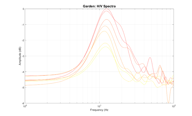
Figure 16 shows the HVSR spectra that were recorded using the 3-component geophone after the sprinkler system was turned off. The colour sequence starts at red and progresses through to yellow following a spectrum sequence. A 30 minute time increment is used between each trace. 9 traces are displayed, conforming to a 4 hour monitoring period. The Log10 of frequency is shown on the x-axis, while the amplitude of the HVSR spectra is shown in the y-axis. The 0.25m loam layer has a natural resonant frequency of around 12Hz. The 0.25m thick loam layer is very thin, yet a clear reduction in the resonant frequency peak can be seen as the loam layer naturally drains of water within its matrix. Another striking result is that the peak amplitude of the resonance reduces significantly in amplitude as the loam layer drains.
Simple metrics such as the root-mean-square (RMS) amplitude of recorded data traces can be used to monitor for soil saturation. The geophone was planted on the surface of the lawn during the experiment which meant that water droplets falling onto the upper surface of the geophone would generate broadband signals during the wetting process.
Figure 17 shows the RMS amplitude data from vertical geophone seismic and electroseismic recordings. Data are displayed that span the closing phase of the water saturation process and into the loam drainage stage. The data from the vertical geophone component show that the lawn sprinkler was operational up to approximately 18:35. The electroseismic data show that the electro-potential RMS amplitude continues to rise slowly up to 18:35, when the loam reaches its peak water saturation level. The electroseismic RMS data then monotonically reduce in amplitude as the 0.25m thick loam layer slowly drains between 18:35 and 20:45.
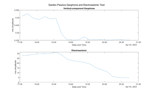
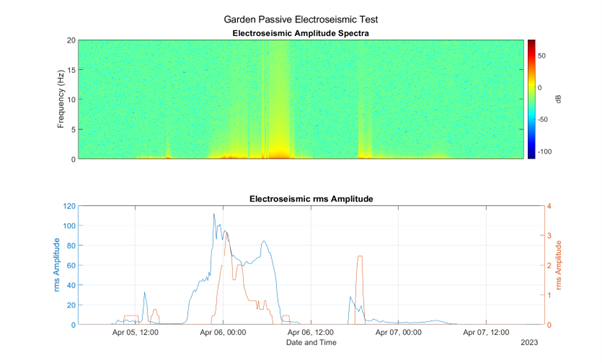
Figure 18 shows an analysis of electroseismic RMS amplitude and spectra data recorded over 3 days when rainfall events were monitored that would increase the water saturation within the 0.25m thick loam layer. Rainfall rate data in mm/hour were obtained from the Cullercoats weather station that is approximately 2 miles from site of the HVSR and electroseismic experiment. The rainfall rate data can, therefore, only reflect an approximation of the actual rainfall at the test site as showers tend to quite localised in both the start and end times and their rainfall rates. The match between the rainfall event time and the RMS amplitude data from the electroseismic sensors, however, is compellingly close. The minor rainfall events lead to a modest increase in electroseismic amplitude. The prolonged rainfall event between 18:00 on April the 5th and 06:00 on April the 6th results in a much higher electroseismic RMS amplitude, as the higher water saturation of the loam leads to high amplitude electroseismic signals being generated. The electroseismic amplitude spectra show that the bandwidth of the electroseismic signals also increases for higher loam saturation levels.
The use of HSVR in combination with co-located electroseismic sensors provide a powerful combination for the monitoring of the near-surface water saturation. The HVSR approach measures changes in soil density while the electroseismic approach measures changes in soil conductivity as soil water saturation changes. Both measurements can be calibrated to allow prediction of when soil water saturation approaches dangerous levels that would cause the soil’s shear strength to reduce, increasing the risk of a landslide.